In February 2018 I started writing some data structures in Rust. Over the previous year I had done small things in Rust, and I’d been a fan for a while. This was a tough project, and gave me the opportunity to learn about lots of new subjects. This project is one of my favorites because it does interesting work, the operating principles are nothing more than the leverage provided naturally by trees, and the implementation consists of straightforward operations on arrays. I’ve explained these data structures on different occasions, and people remark that the mechanisms are understandable and intuitive. I’ll describe what these data structures are useful for, how they work, and point out some of the relevant history.

I wrote trees that work as vectors, and trees that work as hashmaps. They can perform all the usual operations and they can fork into two independent trees. Each of these two vectors/hashmaps can themselves perform any operations, including forking. All these forks are logically independent: doing operations on one fork has no effect on the others. Code operating on one fork is not concerned at all with what is happening or will happen to other forks. Even if threads are concurrently operating on forks, there is no interference and no thread waits for a lock or for anything else: it can always make forward progress. Any individual operation, including forking, completes in a small, bounded amount of time, even as the vectors/hashmaps grow to millions of items. As I’m sure you can guess, although the interface presents logically independent trees, the trees in fact share chunks of memory, parts of the trees that are consistent across forks.
This logical independence is strong. It should be noted that it is inappropriate for some tasks. It separates the data structure writer from which memory will be used to form the updated structure. For some code in a driver or a kernel, the purpose is to drive the machinery, to write bits to specific addresses, so any indirection is completely antithetical. For other tasks, the ability to fork is not giving you new leverage over the problem. Things like networking code, compression, encryption, numerical subroutines, filesystems, database engines, compilers, graphics and multimedia, games and simulations and so much more, largely don’t get any easier to code by forking data. It is more mechanistic and linear, and don’t have need of forking, snapshots, speculative updates etc. I want to be clear that this is not a clarion call to replace working code or use these trees everywhere now.
So when could this logical independence be useful? When I first saw these tree recipes, it felt like a gimmick. I had never once while programming felt the sudden urge to "fork" some data structure. The thought had never occurred to me. All my programs worked without such a thing; clearly it was a bauble, nothing more. But I ended up finding some nice uses for them and being successful. It is useful for tasks like dealing with data coming from other systems, processing information from disk or network, high level decision making, routing to different components, and business logic generally. It works well for tasks that are not the innermost loop of the computation, but the surrounding logic, what I would call "scaffolding": testing, feeding data into core computation, analyzing results, and top level orchestration.
Why I like ints
int x = ...
... = f(x ...)
... = g(x ...)
... = h(x ...)
I get a nice feeling working with ints.
If I’m trying to figure out what will happen with h(x),
I don’t care about what f or g do with x, and it’s fine
if f further passes the value of x on to another function j.
I don’t care what j does.
From the point of view of x, the order of f and g is not
pertinent. Earlier uses of x don’t change its meaning for later uses.
x means exactly what it meant the last time it was assigned.
The activities of intervening code have no effect.
obj x = ...
... = f(x ...)
... = g(x ...)
... = h(x ...)
This feels different. obj here is some heap memory: mallocd or
garbage collected. In some languages, subroutine invocation may be
phrased as method calls like x.f(…), but it’s all the same.
If I’m trying to figure out what will happen with h(x),
I should understand what f and g do with x.
And if f passes x on to function j,
I should go understand what j does.
The order of f and g may be important for x.
Perhaps f changes some contents of x, and g relies on that.
obj x = ...
... = f(y ...) // notice it's y
... = g(y ...)
... = h(x ...)
When heap structures are connected, you may need to understand
code that doesn’t obviously use x.
You may have memory like this:

So operations done to y in f(y) or g(y) may effect the
meaning of h(x).
In Java, you can declare something final. Notably the slot is final,
it will never point to a different heap location, but the contents of that
heap memory can still change.
In C++ and Rust, you can give a "read-only" pointer,
when appropriate.
... = f(&x ...)
... = g(&mut x ...)
... = h(x ...)
In this case it is clear f won’t alter the contents of x,
and it can pass the read-only pointer on to function j, which also
won’t alter x. Demarcating where mutation happens, and defaulting to
read-only, is great, and very helpful for understanding, and I advocate
for using these markers.
We’ll still need to understand what g does with x, and if it passes
that mutable reference on to function k, we should go understand that too.
These markers don’t give any leverage however when there are logical resource conflicts. One part of your program wants to remember, to hold onto some bits, some information exactly as it is, and another part of your program wants to compute new information based on the old.
If you are writing f, and encounter some condition and you want to
remember x exactly as it is right now, remember it for later,
how can you achieve that?
Clearly, you could just make a bit-for-bit full copy of x.
For small things, and in some codepaths, this is perfectly appropriate.
For other codepaths and sizes of data though,
full copy can be unappealing or a complete nonstarter.
You can’t just save off the pointer. After f returns, the caller may write and/or
free that memory. Garbage collection or reference counting can make sure memory isn’t
freed out from under you, but the memory can still be over-written.
An exclusive lock, or a reader lock, can enforce turn-taking, but can’t be used
as a general purpose mechanism for remembering.
Would-be writers are blocked.
Clearly, remembering must involve retaining all the existing bits somewhere. Treating the bits as read-only is easy enough, but then what should a writer do? It shouldn’t over-write existing bits, so it should use some new space to represent the new information. As before, you could make a full copy, and perform all the writes you want on that. But it’s a big up-front cost. If you only end up writing to 5% of the existing data, then copying it all feels like overkill. Some kind of diff would be better. Keep all the old bits read-only, and represent new stuff with a little bit of new space, representing the differences or changes made on top of the old data. A diffing scheme should only take a small amount of new space to represent a small number of changes. At the same time, it should support efficient element access. You can break up memory into pieces, instead of using one big chunk. For instance if you split it into ten equal sized pieces, then updates can operate on one chunk without needing to touch the other nine. This is a good granularity of change for smaller data structures, but when a collection has many thousands of items, 10% is still quite a lot to copy. A tree provides layers of splitting, and so can scale gracefully to large sizes. The strategy is to represent the difference between two trees, by copying a path from root to leaf.
What does this mean for programming with these constructs?
val x = ...
... = f(&x ...)
... = g(&x ...)
... = h(x ...)
Here, val is something that won’t change out from under you. Assigning to
x is the only way its meaning can change. Ints fit this description.
So do these forking trees. There are no &mut operations on the trees,
only read operations and write operations that take ownership of the tree.
Sort of like if you were getting a garment altered: you’d hand the garment over,
they use the existing cloth and maybe some new cloth to construct what you asked for,
and hand you back the result. The write operations take a tree (vector/hashmap) and
return a tree reflecting the desired edit. Commonly, write operations will not
need to use any new memory at all, and will just perform the operation in place,
and end up handing back the same memory address you passed in. But this indirection
is what allows different parts of the program to make independent, runtime decisions
about remembering and editing data.
Write operations are always ready to use some new memory if required because
a fork needs the old memory kept around, even though commonly it won’t need to.
And if I’m writing f, I can do anything I want
with &x, including forking and editing, or remembering.
And in any of these cases, there is no deluge of work that somebody needs to go do.
Nobody is screwed.
If you toss a rock into a stream, the water flows around it.
If f encounters a condition and decides to remember x,
the rest of the program gracefully goes around.
It respects the need to keep x as is, and
works around that, using new memory as required.
These trees by design are not coordination points: you can alias them, or you can edit them in place, but not both. And a coordination point must do both. Well, so what should you do when one part of your program wants to put something somewhere so that another part of your program can see it? The trees don’t do this part of the job. You use a mutable slot, which holds a value (eg one of these trees). You can compute a new value, and stick it in the slot, over-writing the old value. Other parts of your program that share or alias the slot can now see the new value. The slot contains different values over time, but the values themselves are timeless. They don’t vary with time. That’s their whole point.
This is a very different situation from sharing and mutating a data structure. One part of your program wanting the data structure to stay still as it reads, is fundamentally at odds with another part of your program wanting to update it. They must take turns; readers block writers and vice versa. You can’t remember a particular state of the data structure without performing a full copy. But for instance, if I retrieve a tree from a mutable slot and then want to perform a bunch of reads on it, am I in anybody’s way? Other readers can join me in reading the tree, no problem. Are writers stuck waiting? No, they will use new space as required to represent new information. These writes never disturb readers, who always see a consistent snapshot. A writer could take a new tree and save it to the slot. This publishes the new info for future readers and writers, but in no way disturbs ongoing computations against the old info.
Dynamic
The scenario of one part of your code wanting to remember even as another part wants to compute new things, is a pretty static situation. But it also works for completely dynamic situations.
What if your program would like to pass data to an unknown number of handlers, which could be functions added to a list at runtime. No problem; if there end up being 4 or 40 handlers that each need the data, you just make 4 or 40 forks as appropriate, and give each handler one fork. In these handlers receiving a fork, the code doesn’t know or care if there are other forks or what other handlers might be doing with them. The code is also free to do anything it wants with its own fork: read it, write it, pass it on to other functions, remember it. And whatever it chooses to do, it won’t disturb the other handlers or get in their way.
Not only can remembering something be a runtime decision, but a debugger or instrumentation facility could trigger remembering a value at any point in user code. These facilities could inspect locals and perhaps choose to remember some of them. Signaling this amounts to incrementing a memory cell, a counter. Then it could return control to user code, which will happily march forward. It is undisturbed by this unforseeable decision to remember something. Having incremented a counter, the vector/hashmap (all the bits that make up the tree) will stay exactly as it is, indefinitely. At any point in time later (milliseconds or days), the debug facility can revisit the remembered tree, and find it exactly as it was, and the program moving forward in the meantime had no effect on it.
You could share these trees with C code.
Imagine a Rust program dynamically loads a C module, and passes a tree to
one of the C functions. In C, this would probably be represented as a
typedef around void*. Imagine you are writing the C function that receives
a tree from the Rust code. Do you care if there are forks of the tree, being used
by other Rust code, possibly even in concurrently running threads?
No, and you also don’t care what the Rust function will do after you return.
Symmetrically, the C code is free to do anything it wants with the tree, including
reading, writing, forking, remembering, and passing it on to other C functions.
None of this will disturb or mess up the Rust code; it doesn’t know or care what
the C code ends up doing with the tree.
Points and comparisons
Rust has three modes of passing parameters: read-only pointer, mutable pointer, and handoff of ownership (called "move semantics" in C++). These trees don’t provide any mutable pointer operations. Otherwise they are unremarkable Rust types.
The implementation of these trees is couched entirely in terms of arrays. Malloc and free, get and set index, and basic arithmetic are all that’s required. I believe these algorithms on arrays would be readily portable to C, FORTRAN etc. I would hope another C programmer would look at the Rust code for these tree operations, and see what I see: function for function, line for line, exactly what it would look like in C. There is almost no semantic gap.
There isn’t any pressing need to port these trees, but I do appreciate that the algorithms work on generic building materials. The in-memory layout of these trees of arrays is straight forward. It is easy to imagine code written in other languages that could traverse these heap structures at runtime, or in a core dump.
Rather than over-writing data in place, ZFS uses new space to represent new data. This completely changes the paradigm. Data is always consistent, using transactional copy-on-write. Snapshots and (writable) clones are cheap. Clearly, there is some resemblence between these forking trees and ZFS. However, ZFS takes on a big job and manages many different storage media, whereas these trees address a comparatively constrained problem operating only in RAM. So I wouldn’t want to push the metaphor very far. That said, the basic principles at work are familiar.
This is a diagram from the paper showing how ZFS represents a new filesystem tree as a small difference from the old tree, by copying along the path from leaf to root. It could just as well be a demonstration of the in-memory trees forking. Using differences between trees makes keeping snapshots cheap. It also makes remembering an in-memory tree cheap. And a writable clone is similar in spirit to forking these in-memory trees. An interesting difference, the in-memory trees do overwrite chunks of the tree, when there are no outstanding snapshots/clones that need it. So while a tree is always ready to copy some parts along a path, for the vast majority of the writes in realistic programs I can imagine, it won’t end up copying at all, just mutating existing memory in place. This doesn’t make sense for the ZFS disk structures, but I think it’s a nice fit for RAM.
Version control systems don’t overwrite historic data, and often represent new data as a diff or delta from the existing data. Branches (which may share common history and artifacts), are functionally independent, and activity in one branch does not effect others. Clearly, there is some analogy to be drawn here with the forking trees. The ability to hold onto the past without impeding writers is important. And so is the independence of writers across branches.
Some systems allow you to try out some edits without trashing the existing data. This could be for answering "what if" questions. It could also be to try before you buy (commit) to changes, or to make a group of edits transactional. In some contexts it might make sense to keep a log of edits, such that you could decide not to keep the edits, and one by one change each edit back. This won’t work if there are multiple threads of control, and can’t support remembering. These forking trees work much more like ZFS or MVCC that accomodate readers and allow writers to move forward via diff, and a commit looks like changing a mutable slot from the old tree root to the new tree’s root.
Systems using ref counting and malloc can have certain pain points. Cycles are a thorn in the side of ref counting. Systems deal with this by integrating occasional sweeps that can collect cycles in memory. These forking tree structures cannot form cycles, so sweeps are not needed. A core challenge in a non-moving memory allocation system (like malloc), is to avoid wasteful fragmentation. The worst cases for fragmentation are unavoidable when the range of sizes requested vary widely from smallest to largest. Real programs may certainly request memory across many orders of magnitude sizes (eg 10 bytes up to 10 million bytes). These tree data structures never allocate giant chunks of memory; everything is broken up into a somewhat small sizes (eg 1-8 cache lines of malloc’d memory). Even though there is no memory compaction, using all small sizes makes fragmentation less pernicious.
Is reference counting a form of garbage collection? Certainly in some sense. But I think of garbage collection as a system that periodically (but unpredictably) sweeps over the stack and some parts of the heap. Resources are not released predictably. This strategy emphasizes overall throughput, but suffers from pauses. Many modern garbage collectors break up the work, making pauses much smaller, at the cost of some throughput. These forking trees do use reference counting, but it doesn’t feel like garbage collection to me. It feels like a library, not a framework.
Although this scheme does runtime dynamic memory reclamation, it
is prompt not delayed. When user code is done with one of these data
structures, the drop code will promptly reclaim all parts of the
tree that are no longer needed.
Notably, you can always choose to delay it.
For instance if you are in a critical path to answer a network request,
you could hold on to large trees until after you have sent a response,
and only then drop the trees and incur the cost of tearing them
down and reclaiming their memory.
Code that has one of these trees in hand, has the absolute promise that the exact bit configuration of all memory deeply down the tree will remain untouched indefinitely. This includes the elements in the vector/hashmap, they won’t change either. And if an element is itself a container, the items inside it are also unchanging. All memory reachable from the root of the tree will remain unchanged. Critically, this is not a lock. If there are other forks, they are not impeded: if they want to write they will move forward without disturbing others. Unlike a mutex, nobody is ever locked out. It’s somewhat like a readers lock: any number of readers can coexist. But unlike a readers lock, writers never wait for readers: they just move forward without disturbing readers. Of course, this is a form of reference counting, and also a type of semaphore. The special rule is that if the count is more than one, then the memory is effectively read-only. If the count is exactly one, an edit operation can feel free to modify the memory, since nobody else is relying on it.
Amortized strategies optimize for overall job throughput, at the cost of latency outliers. With garbage collection most allocations are cheap, but every once in a while an allocation takes a very long time. Vectors and hashmaps have something similar: adding to the collection is usually cheap, but sometimes adding one item requires first copying all existing items (to a new, bigger, monolithic chunk of memory). In practice this isn’t much of a problem, because either the collections are small and copying them occasionally doesn’t matter, or the collections are large but we only care about overall throughput. So this is not a pressing matter, but it is interesting that the trees are deamortized. Any operation on a tree, no matter what the forking situation is, has only a small amount of work to do. The key to this is breaking up the monolithic chunk of memory into a tree. Growing or shrinking the tree is graceful and never requires a rebuild. That’s the essential leverage of the tree.
The term "copy on write" makes for the unfortunate acronym COW. In-memory copy on write structures often mean "copy entirely on every write". I avoid using such data structures even though they can be useful. It feels wasteful, and unnecessarily precautious. These forking tree data structures copy only as required to differentiate multiple forks. And in particular, if a program doesn’t fork any trees, no copying will be required. This pattern of usage feels sufficiently different to merit a new moniker. I think "copy on write as required" COWAR is just as uninspiring. And "copy on conflict" could be misunderstood (confused with the proof assistant). So I would prefer to refer to this strategy as CAR, copy as required.
Vectors
The vector trees can have an arity (splitting factor) of 16, 32 or 64. This is a tradeoff between access performance and write granularity. A 16-way tree is a bit taller (more indirections for access), but if a write operation must copy, it copies a narrow, more targeted path down the tree. A 64-way tree is shorter (fewer indirections), but writes are less granular. Less granular writes are not always a problem; if you are going to write to many of the other 63 elements at some point, might as well pull them all in up front.
The 16-way trees are the best for illustrations though. In the diagram below, we can see a vector data structure growing as more items are added to it. The lighter shaded boxes indicate unoccupied memory. You can see that as items are added, the vector will resize to larger and larger memory chunks, until it hits the arity limit.

The array labeled "A", holding the 17th element, is the "tail" of the array. The tail is the business end of the vector, and most pushes and pops don’t involve the tree proper, but just add or remove an element from the tail.

Each array records its size and reference count in the first unit, drawn as a circle. Pointers to arrays are pointers to this self descriptive information. Next is the virtual table; it’s drawn as a triangle, since the table is an indirection that reminds me of a prism refracting light. The triple bar hamburger menu holds the element count of the vector, five in this case. And we can see five array positions occupied.
At 17 elements, the vector grows a tail. Once that tail fills up, the tree grows in height, moving the contents of the root out into its own array.

As more elements are added, tails fill up one by one and are added alongside the other fulls. Once the root grows till it hits the arity limit, it’s time for the tree to grow in height again:

A tree with four of those 16x16 blocks completed:

A tree that is very close to growing in height:

You can see here each grouping of 256 elements is drawn together in a tight block. The 16 arrows leaving the root each conceptually connect to one of the 16 blocks (it’s just messy to draw). If you add 16 more elements to this vector, it will grow in height, moving the root contents out into its own array.
In the tree above, you can see that accessing an element requires following two pointers starting from the root. A tree that requires following three pointers can address 65 thousand elements. With four levels below the root, it can address one million. See the table below showing for each tree arity (16, 32 and 64) how many elements can be addressed based on the tree height:
Levels below root |
|
|
|
1 |
|
|
|
2 |
|
|
|
3 |
|
|
|
4 |
|
|
|
5 |
|
|
|
6 |
|
These data structures are trees, but they’re pretty flat. Accessing one element out of a hundred thousand follows only two pointers. And a tree with hundreds of millions of elements is only a handful of levels deep.
Vector implementation
These tree designs may be simple enough now, but in fact I started with complicated schemes in a huge design space, and laboriously whittled my way down. After weeks of planning, I started an implementation, and quickly failed. The strategy was not working, and the code was very hard to understand. No problem, back to the drawing board. I came back weeks later with another grand design, and again, after several days of quagmire, concluded I was writing code that I wouldn’t be able to reason about effectively. One false start is no problem (prototype and course correct) but I’m not used to getting stuck twice. I had to get it right for the third try: I strengthened the array constructs and built out subroutines for manipulating arrays. The third time was the charm, and I finally created an implementation that I could understand, debug, maintain etc.
When the assertions are enabled, all arrays are zeroed upon allocation, and zeroed after being freed. Reads and writes are bounds checked, and writes additionally check that the reference count is exactly one. Bit patterns that are expected to be pointers to an array can check a redundant bit pattern in memory, to guard against treating junk bits as a pointer. None of these dynamic checks are necessary, assuming my code is bug free. They act as a guardrail to detect errant machine state and fail early, to help me fix the bug in the tree code. They do not impact library user code, and someday it might make sense to turn these guardrails off for some builds (for a bit of performance boost).
The implementation is probably not too surprising, but there are a few interesting things to point out.
pub fn conj_tailed_complete(guide: Guide, x: Unit) -> Unit {
    let tailoff = guide.count - TAIL_CAP;
    let last_index = tailoff - 1;
    let path_diff = tailoff ^ last_index;
    match digit_count(last_index).cmp(&digit_count(path_diff)) {
        Ordering::Less    => { growing_height(guide, x, tailoff) },
        Ordering::Equal   => { growing_root(guide, x, tailoff) },
        Ordering::Greater => { growing_child(guide, x, tailoff) },
    }
}
The code above decides which case we are in, based on logic similar to an odometer rolling over. If adding one only changes some of the digits, like 859 → 860, then we will grow the tree by adding to existing arrays below the root. If adding one changes all the digits, like 899 → 900, then we will expand the root. If adding one results in more significant digits, like 999 → 1000, then the tree will grow in height. The width of a digit is 4, 5 or 6 bits, depending on the arity.
In several places, you’ll see code like this:
if s.is_aliased() {
    let t = Segment::new(size(grown_digit + 1));
    let range = s.at(0..grown_digit);
    range.to(t);
    range.alias();
    if s.unalias() == 0 { // Race
        range.unalias();
        Segment::free(s);
    }
}
An array of memory is aliased (ref count more than one), so we copy it. Now we are done with the original, and unalias it (decrement its ref count), but find that the count is now zero! This can only happen when multiple threads are actively working on the same memory. While the first thread was copying, a second thread decided it was done with the array and decremented the count down to one. Then the first thread comes back, decrements, and finds nobody depends on the original array any more, and it must clean up. So it frees the array. If these conditions were not included, racing threads could end up subtly leaking memory.
It’s pretty challenging to imagine how you’d test that these code paths do what they should, and that you haven’t forgotten some. Obviously, you could have threads race over and over, checking for leaked memory, and hope you stuble upon proper conditions to trigger these race conditions. That can’t be the whole story though, so last year I worked on a testing harness to systematically explore thread interleavings. It instruments certain critical array operations, forcing a pair of threads to deterministically follow a predefined schedule of turn taking. How schedules are explored takes inspiration from CHESS (2008). If a problematic schedule is found, it can be rerun at will to visit that same thread interleaving (and confirm you fixed the problem). This worked out well, and all the tricky code paths could be triggered with low complexity schedules. But it doesn’t help find missing paths I don’t know to look for. For that I’ll need to someday do automated generation of tree scenarios, and then systematically explore possible schedules for each. This would be reminiscent of my project testing Java priority queues.
Another way to provoke use of these code paths is to have the implementation
of is_aliased() occasionally lie and report an array is shared (count over one),
when the count is actually one. This lie makes the writer perform an ultimately fruitless
copy, and then clean up the original after it decrements and finds the count to be zero.
This lie is logically harmless, and just inspires extra work exercising these
seldom needed code paths.
-
conj is for adding (pushing) a new element to the tree
-
pop is the inverse of adding to a tree
-
nth is access by index
-
assoc is write by index
-
reduce is a traversal of the tree that feeds the elements into a stateful aggregator
-
tear down is a traversal over the parts of the tree that are no longer needed, and can be freed
-
eq is a traversal over two trees in tandem, comparing elements for equality, and of course short circuiting on any parts that the trees share
Maps
The map trees can have an arity of 16 or 32. Since elements added to the map are pairs (key and value), the biggest array sizes used are 32 or 64, respectively. Again, the tradeoff is between access performance and write granularity. The 16-way trees are convenient for demonstration, since the digits are hexadecimal.
A key is hashed and the hash informs where in the tree it will be stored.
Imagine the hash is B10F3A78. The first digit is B.
If the B slot in the root is unoccupied, then the key will be stored in the root.
If another element’s hash also starts with B, then both keys will be stored in an
array below the root, where their second digits will be used to differentiate them.
If keys conflict in two digits, then another array and a third digit will be used,
and so on. The keys are stored in order of their hash digit.
In the example below, we start with an empty map and add a key whose hash
starts with B, then add a key starting with 5, then one with 7, F, and 4:

The tree at size 6 shows an array being used to store two keys,
both of which start with B. One’s hash is B1------ and the other is BA------.
The tree at size 7 adds C to the root.
And at size 8 we see another array being used for two keys: 56------ and 5D------.
After a few more additions, the tree looks like this:

Notice in the root the three arrays are ordered (5, 7, B)
and the keys are ordered (4, C, F), with the arrays grouped at the front.
This tree has quite a few keys starting with 7, and two of them start with 7E:
both 7E3----- and 7E5-----.
(Keep in mind that this distribution of keys is not very likely. I picked it to show a multi leveled tree. In practice the average tree has a pretty wide fan-out.)
So how do we navigate the tree? The squares that look like dice hold a bit array, marking which digits are present. Next to the triple bars, the bit array marks what is present in the root:

If you need to access the array 7, you count up the array bits before 7, which
is a mask and a pop count. Only one bit, the array 5.
So the offset of array 7 is one pair from the front.
And if you need to access key F, you count all the array bits (3)
as well as the key bits before F (2). So you can find key F five pairs
from the front.
And, as you can probably guess, the bit array associated with array 5
marks which digits are present in that array. Same for arrays 7 and B.
I took a list of 84,000 words and randomly selected 500 to put in a 32-way
tree. The diagram below shows the part of the tree that holds hashes starting
with C, 20 keys total. The other 480 keys are stored in the other 31 arrays.
In base 32, the digits go 0-9 and A-V. The bit array shows 15 keys present
(1, 5, 6 etc) and two arrays (8 and T).

Keys like "evacuee" are unique after two digits, so accessing them means traversing one pointer from the root. 62% of the keys in this tree reside one level below the root, and another 36% are two levels below the root (like "fallibility"). So a total of 98% of keys can be found by following one or two pointers.
Lookups of keys that are not in the tree are called "unsuccessful".
We can expect 60% of unsuccessful lookups to halt after reading the root,
since it has bit arrays describing 1024 (32 squared) two-digit patterns,
and only about 40% of the two-digit patterns are present (395).
In this case you don’t follow any pointers.
For example if a key hashed to CJ-----, we could know it is not present
and halt the search by reading the C bit array in the root.
Here are the keys whose hashes start with D and with E:

For the same 500 words in a 16-way tree: 85% of keys require following two or fewer pointers, and 99% follow three or fewer. For the 32-way tree with all 84,000 words: 92% of keys follow three or fewer, and 99% with four or fewer. For the 16-way tree with all 84,000 words: 28% in three or fewer, 92% in four, and 99% in five.
500 |
84k |
|||
Levels below root |
x32 |
x16 |
x32 |
x16 |
1 |
62% |
14% |
||
2 |
98% |
85% |
8% |
|
3 |
99% |
92% |
28% |
|
4 |
99% |
93% |
||
5 |
99% |
There are tons of useful maps that use 500 keys or less; most keys are located by following one or two pointers. To me, this feels very different from using a binary tree. The tree is decently flat.
Ditto for maps with tens of thousands of keys; most keys are located by three or four pointers. This is palatable, and feels more like a hash table than a binary tree.
Map implementation
The implementation is, perhaps unsurprising, all about shuffling things around arrays. Here is the loop that descends, level by level, in order to find the right place in the tree for a new key to reside:
for idx in 1..MAX_LEVELS {
    ...
    let digit = digit_at(hash, idx);
    if pop.array_present(digit) {
        ...
        continue; // down to next level
    }
    if pop.key_present(digit) {
        // collide with pre-existing key
        return has_key(...)
    } else {
        // slot empty, add new key
        return new_key(...)
    }
}
It checks the bit array (pop for population), and if an array is
present for that digit, we continue down the tree another level.
Otherwise, if a key is already present with this prefix of the hash,
we differentiate the two in a new array, one level below.
And if the digit is not present altogether, then we’ve found the
right place for this key.
A small point to note, this same tree can act as a hash set: only keys and no associated values. The keys are grouped up together with no gaps, and all calculations account for this.
-
assoc is adding a new key into the tree
-
dissoc is the inverse of adding to the tree
-
get is access by key
-
reduce is a traversal of the tree that feeds the elements into a stateful aggregator
-
tear down is a traversal over the parts of the tree that are no longer needed, and can be freed
-
eq is a traversal over two trees in tandem, comparing elements for equality, and short circuiting on any parts that the trees may share
Forking
Below, there is a digram of a tree that will demonstrate forking.
For simplicity, I’m not showing any meta information or tails.
Imagine we want to change the contents of index 0x1A, the blue cell
in the array labeled B, but someone else wants to remember the original:

We would copy the root (labeled A) and the array B.
The copies are shaded darker. They are bit for bit copies,
except for the colored cells. The original tree contains
the blue element, and the new tree contains a red element at index 0x1A.

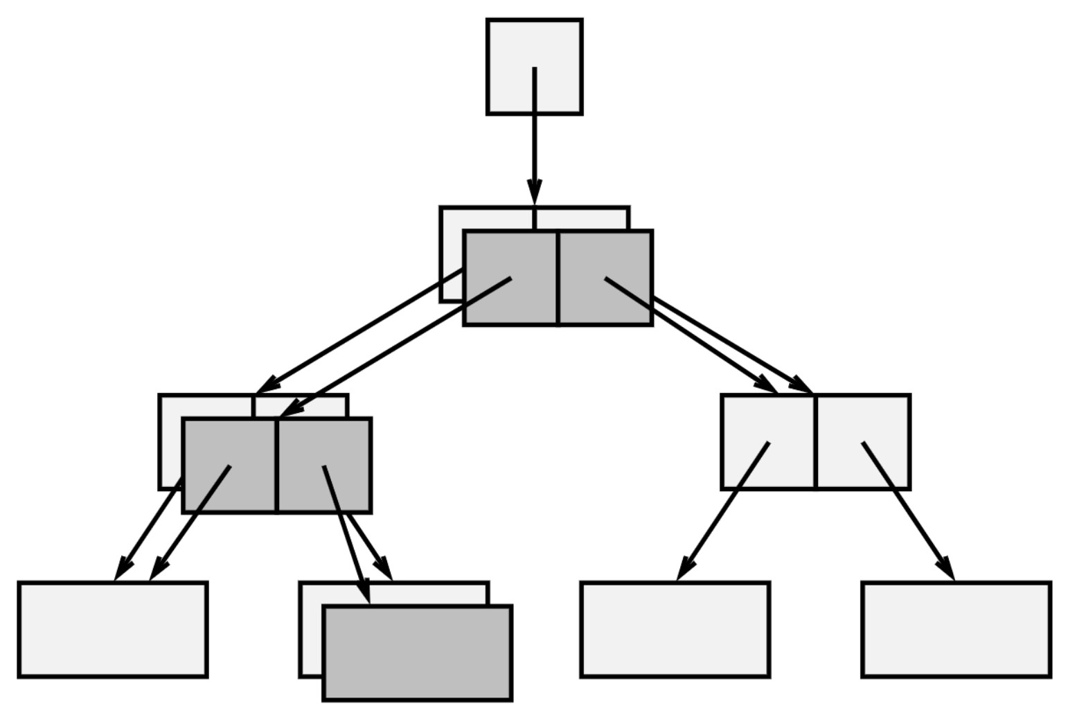
The same situation on a tree with over a thousand elements:

We want to change the blue cell in array C, but someone wants to remember the current tree. So we’ll copy A, B, and C:

Below is a blow up of the same diagram. Note that a second write operation won’t need to copy the root (A') again; that’s a one-time upfront cost. A write to the contents of array D will only copy D; A' and B' will be reused. A write to the contents of C' won’t do any copying at all.

Forking the hash map tree works just like this. The path from the root to the key is duplicated.
Plans
What was the point of writing these data structures? What’s the big picture? I found these techniques (forking trees) really useful in the JVM. But often I needed to work in other places. And while most languages nowadays have one or more projects for providing persistent data structures, they are inconsistent between languages, partial, and idiosyncratic to fit in with the current language. People can and do use them successfully, but I would characterize it as pulling out the special fancy dinnerware once a year. Much of the benefit I saw when using them in the JVM was because they were everyday workhorses, and large sections of logic in a program could be phrased in terms of these sturdy components. What I really want is a (cross language) library of values: a consistent, high quality experience across languages, and wire formats that make passing data between languages seamless and lossless.
A consequence of this goal is that the library should be cohesive and self-sufficient, with minimal requirements on the hosting environment. In particular, it should not need a garbage collector. It is wholly unsatisfying to a C programmer or similar, to hear that a "library" needs to integrate with a collector framework, or worse, invites you to participate in its own framework.
Many things could be built atop a library of values, general data processing
and the like. The benefits mentioned in the introduction apply.
Code can share around data without worry of interference, logic within functions
is largely independent of the logic in other functions, and is robust to changes
made in other parts of the codebase.
Any arrangement of data usage or remembering within a program is valid,
even when dynamically decided.
Concurrent, asynchronous, or even parallel usage of data is easy to reason
about, since it follows a strictly textual and sequential model.
Working with large data aggregates feels like working with ints.
Of particular interest to me is building a "database engine in a box". SQLite is notable for embedding the query engine inside the application. There is a particular database model which uses redundant storage of unchanging artifacts. While there is a single special machine in charge of processing new transactions, any number of machines can query and analyze the data from a particular moment in time. Since the underlying data chunks are unchanging, it is perfectly reasonable to perform long running queries or analytics on a machine. The data won’t change out from under you as you compute, and a box performing long running computations in no way interferes with other machines performing queries nor with the special machine accepting transactions. This is possible by separating out the portion of the database system that accepts transactions from the parts that query or analyze data. And in particular, any number of client applications can embed their own query engine and participate as first class peers in a database system. You can also imagine an application using a static database, with no connection to a live transactor, only computing on an existing set of unchanging artifacts. And of course, these unchanging static assets are perfectly amenable to any caching strategy, and could be readily hosted on a CDN for example.
Again, I want this embeddable query engine to function as a library, not a framework, and it should make sense across a variety of languages. WebAssembly is a high quality sandbox (building on work such as Sandboxing-JITs 2011 and Native-Client 2009) that is available in many languages and environments. A proper query engine should support truly ad hoc queries and data processing. And it should compile custom code paths on demand (rather than interpreting graph structures or bytecodes). To this end, I’ve designed and (partially) prototyped an interactive WebAssembly compiler that dovetails with this model of forkable data structures.
Click on the text in the box below. Clicking it starts a web worker, which will use a WebAssembly runtime to process commands.
(conj (conj (conj [] 7) 8) 9)The run button sends the text in the box over to the worker, which
feeds it into a wasm function. The wasm code parses a well known data exchange format
(basically ints and floats, strings and names, vectors and maps, and a few other goodies),
then it resolves names and compiles a tiny wasm module.
The tiny module (234 bytes) is loaded into the same runtime as the mothership module
(the data structure code and compiler), and then it is executed.
It calls a function in the mothership to produce an empty vector,
then calls other functions to push numbers into the vector (conjoin).
The end result is a vector of three items. It is printed as [7 8 9] and sent
from the worker to the main thread, which displays it.
The text below shows how my browser’s debugger displays the tiny module’s code. The instructions operate on an implicit stack, much like RPN calculators or Forth.
(func (result i32)
  // fress is the mothership module
  call fress.new_vector
  i64.const 7
  call fress.from_i64
  call fress.conj
  i64.const 8
  call fress.from_i64
  call fress.conj
  i64.const 9
  call fress.from_i64
  call fress.conj
)
The design supports a very small, orthogonal language for arbitrary computation. The implementation currently only has facilities to call the three functions seen above, and so can’t do much more than the above example. But it shows the core operational activities: a mothership wasm module is loaded into a fresh sandbox/runtime by a host, commands fed into the sandbox are parsed, understood as a program, compiled to a wasm module, loaded into the runtime, executed, and results returned to the host.
Benchmarks
It is important to measure my tree data structures against other existing designs;
it is not enough to just have nice sounding ideas.
First, I compared the map trees against Rust’s HashMap,
which since version 1.36
(stable in July 2019) uses the hashbrown implementation
(a variant of Google’s C++ SwissTable, presented in 2017).
Often, people benchmarking hashmaps will use integers as the keys. I care much more about the case where the keys are (somewhat short) strings. I used a shuffled list of 84 thousand distinct words, appending sequential numbers onto them as needed to create more distinct strings:
static WORDS:      &str  = include_str!("words-shuf.txt");
const  WORD_COUNT: usize = 84_035;
fn words() -> impl Iterator<Item = String> {
    WORDS.split_whitespace().map(|w| format!("{}", w))
         .chain(WORDS.split_whitespace().cycle()
                .zip((1..).flat_map(|n| repeat(n).take(WORD_COUNT)))
                .map(|(w, i)| format!("{}{}", w, i)))
}
// words() => humbler,  unmanned,  bunglers,  ...
//            humbler1, unmanned1, bunglers1, ...
//            humbler2, unmanned2, bunglers2, ...
People often try to isolate the latency of an individual operation. I care more about end to end performance of a mixture of many operations. To this end, I measured the performance of a hashmap on an "obstacle course". Given the number of keys to use (eg 100), it takes an empty hashmap and associates each key with an incrementing number:
let mut m = HashMap::new();
for (i, w) in words().take(count).enumerate() {
    m.insert(w, Value::from(i));
}
Then it:
-
loops over the words four times, looking up the associated numbers and summing them, checking at the end that the correct sum is computed
-
takes a quarter of the words and reassociates the keys with the sum number
-
performs unsuccessful lookups (eg 100)
-
takes another quarter of the words and removes them from the map
-
and finally drops the map, recovering all heap memory
The code for the map (and set) benchmarks is here.
This medley of operations gives just one data point about performance, so we should take it with a grain of salt. We could argue about the relative proportions of the operations in the mix (eg successful vs unsuccessful lookups). It is also apparent that this medley does not address performance of operations when the hashmap is cold, which must be measured by interleaving with other activity in between hashmap operations. But I believe that this data point is not entirely untethered from what real programs do with hashmaps.
There are several different variants that I wanted to measure.
I wanted to test both of the map tree
arities, 16 and 32 way branching. For the Rust HashMap, I evaluated three different hash
functions, and the effect of reserving space vs letting it resize on the fly. The default
hash function is SipHash, which prioritizes resistance to collisions from maliciously chosen
keys over speed of computing the hash. I also evaluated speed prioritizing hash functions:
AHash and
FxHash
(which is what the Rust compiler itself uses).
All measurements in this section were performed on a
2016 i7-7500U
with a base frequency of 2.7GHz (max 3.5GHz), two physical cores (four virtual),
64K of L1 data and another 64K of L1 instruction cache,
512K of L2, and 4M of L3 cache connected to two 8G DDR4 modules configured to 2133 MT/s.
(Eventually I will want to run these same tests on a desktop machine, a server, and something
small like a Raspberry Pi.)
See the chart below:

This chart shows performance on the map medley; lower is better.
The first thing to note: the horizontal axis is the size of the hashmap (number of keys)
on a log scale.
The values are the time relative to the default hashmap
(SipHash and no reserving space) labelled Hash.
You can see that reserving space can improve the time by 7% or more, and using a
speedy hash function can improve time by 10% or more. Using both a fast hash and
reserving space can give a cumulative improvement of 14% or more.
That bump in the tree performance lines is interesting. Note that since it is relative to the normal hashmap, the line going back down after the bump is not indicating it getting faster, just getting faster relative to the baseline. This bump is probably due to a corresponding bump in cache misses over the same sizes. At 64 thousand, you can see that the tree has over twice as many cache misses as the normal hashmap:

The policy around growing the leaves of the map tree is optimistic (double every time), and so a refinement in leaf allocation logic may be able to smooth this bump out somewhat. Back in the original graph, ignoring the bump for now, it appears that the tree’s performance is growing linearly, relative to the builtin hashmap. But remember that the horizontal axis is log scaled, so this upward trending line is actually a slow growing log function. In the worst of cases (for this particular medley), the tree comes in below the 2x envelope (my design target was to be within 5x). And for many useful sizes it is only, say, 40% off the normal hashmap. This is a trade off, giving up some peak straight-line performance for the ability to cheaply fork. Let’s zoom in on the part of the graph for maps under eight thousand keys:

While it is very important that the performance doesn’t fall off a cliff when you get into the large sizes, it is quite common to use maps at smaller sizes: tens, hundreds, or maybe a few thousand keys. So I care deeply about performance in this range. As you can see, for these sizes the tree maps are within 25% of the standard hashmap.
Set performance
The performance for sets is similar. The "obstacle course" is a bit different (naturally). It adds each word to a set (say, 100 words), then:
-
loops over the words four times, confirming that the set contains it
-
performs unsuccessful lookups (eg 100)
-
takes a quarter of the words and removes them from the set
-
adds the same number of new keys into the set
-
and finally drops the set, recovering all heap memory

Unsurprisingly, we can see the same features in set performance. Faster hash functions and
reserving space can give a decent speed up on the default HashSet.
The tree’s performance never exceeds 2x of the default, has a bump around 100k, and for
many useful sizes stays within 40% of the baseline. Here is a closeup of sets with less
than eight thousand elements:

A general note, the HashMap is a generic container given contrete types, and
so the compiler has the opportunity to directly link, and perhaps inline,
operations on keys like hashing, equality and tear down.
By contrast, the trees use dynamic calls (late binding, vtables) for all collection operations
(insert, lookup, remove) and all operations on the keys (hash, equals, drop).
This isn’t the end of the world, obviously, but it’s not making things any faster.
I chose not to control for this difference. I wanted to measure against the most competitive
(and most realistic) configuration.
We could have a map perform an "obstacle course" and save off a snapshot every so often during the exercise, in order to get a sense of the cost. Given a target size, eg 100, I add that many entries to an empty tree, then one by one overwrite each key with a new value, then one by one remove each key, leaving an empty map. Along the way we could take no snapshots, which is the fastest (straight-line performance). Or we could take snapshots every, say, 10 operations. I have the map grow and shrink over and over performing a million operations, so snapshotting every 10 ops would leave us with 100 thousand snapshots at the end. Each snapshot is a first class map that can be used completely independently of any of the other snapshots. So how much longer does it take to create and retain those 100 thousand snapshots versus simply doing the computation and keeping no snapshots?

This graph shows the effect of performing more or fewer snapshots on the time it takes to complete the obstacle course. All times are normalized to the fastest configuration (no snapshots, straight-line). Each line graphed shows the effect for a certain map size. At the top end, you can see that a map of 400 thousand distinct keys can retain a snapshot after every single operation, and the performance is about 10 times the straight-line performance. For a map with one thousand keys, snapshotting after every operation increases the time by 4x.
Take the map with 400k keys for example. It does 1.2 million operations total: 400k inserts, 400k overwrites, and 400k removals. The difference between no snapshots and 1.2 million snapshots is 10x the time and 40x the space (as measured by page-faults). At the end you have 1.2m hashmaps, each is distinct in memory and each is a distinct logical mapping, no two are equal in contents. 400k of them contain 400k keys each, and another 400k contain over 200k keys each; these are not small maps. And each is ready for high performance reads and writes. You can imagine an implementation where a snapshot is a lazily realized view on an underlying data source, making them cheap to create but with poor lookup characteristics. You can also imagine an implementation where a snapshot is fine for reading, but writing would spur a large amount of work. My tree implementations use no such "tricks". Given how much more work it is to create (and later tear down) 1.2m maps than it is to just perform 1.2m operations on a map, it’s kind of amazing it only takes 10 times as long.
More realistically, you often won’t care to fork after every single operation, but maybe after a few dozen or a few hundred operations. And often the maps will hold only dozens or hundreds of keys. Let’s zoom in on maps under a thousand keys:

We can see that a map with 100 keys taking snapshots every 10 operations, takes about twice as long as no snapshots. And for a map with 1000 keys, snapshotting every 10 ops takes a bit over three times as long.
All the measurements so far have used the 32-way branching map tree. How does the 16-way tree perform?

I was honestly quite surprised by these results. I expected to see the wide branching factor tree (x32) be decisively better when snapshots are infrequent, and the more narrow tree (x16) be decisively better with frequent snapshots. As you can see from the graph above, I was wrong on both counts. For maps with 100 or 1000 keys, neither tree is much better than the other at any range of snapshot frequency. I was expecting dramatic differences, perhaps 20% or more. And for maps with 10k keys, the narrow tree is worse at high frequency snapshots and basically equivalent at low frequency!
There are several factors potentially influencing this outcome. First, perhaps obviously, although the x32 tree has to copy wider arrays, it copies fewer of them on a path from root to leaf. More subtly however, the x32 tree has better bit packing efficiency in a 64 bit pointer environment (which is what I’m using). This is because I keep two bits per possible hash digit, meaning 64 bits in the case of the 32-way tree, and 32 bits for the 16-way tree. Since the unit of storage is the size of a pointer, on 64 bit pointer platforms the x32 tree perfectly fits, whereas the x16 tree is leaving half the bits unused. For multilevel trees, this could mean wasting a quarter of the bytes in the (few) nodes near the root. Of course the real cost is not in wasting bytes, but in making those cache lines less information dense.
It is interesting to note the memory usage of the different tree arities. When snapshots are infrequent, both the x16 and x32 trees use the same amount of memory (as measured by page faults). But when taking snapshots every operation, the wide tree uses as much as 50% more memory across different map sizes. Again, this can probably be ameliorated by a less aggresive/optimistic resizing policy for the leaves.
I compared the tree maps with the standard Rust HashMap on a single composite exercise.
To be clear, the trees are in no way a substitute or competitor to HashMap,
and I don’t see myself spending time turning them in that direction.
Their purpose is to work with other code I wrote, and I compared with HashMap
to get a sense of the costs of my approach.
I cannot draw strong conclusions based off my single small benchmark,
but I feel positive about the results so far.
It seems like the trees will be acceptable in performance for the use cases I have in mind.
I evaluated the effect of forking on map performance, again on a single exercise. I found that for realistic frequencies of taking snapshots, the slow down is mild. And when I compared 16-way and 32-way branching, I found they had a similar profile across different snapshot frequencies, with the 16-way tree lagging in performance for larger sizes.
Vector performance
I compared the vector tree to Rust’s built in Vec on a sequence of operations.
First it inserts heap numbers to grow the collection to the target size (eg 100):
let mut v = vec![];
for i in 0..count {
    v.push(Value::from(i));
}
Then it:
-
accesses every other element (the even indices) and sum them all up
-
saves that sum to every third position in the vector
-
pops a quarter of the elements out of the vector
-
and finally drops the vector, recovering all heap memory
The code for the vector benchmarks is here.
Again, this medley gives just one data point and so can’t be used to draw broad conclusions.
I wanted to evaluate a default Vec and Vec::with_capacity
(reserved capacity). What I found was not at all what I expected:

Pre-allocating the exact right size actually made things slower for most sizes;
I had predicted that it would speed things up.
And the default Vec exhibits sudden changes in performance depending on the size;
those little "table mesas" are not artifacts of measurement, they are repeatable and
have hard edges where increasing the vector size by one will cause a dramatic change in time.
What the heck is going on?
Well I noticed that on some sizes, the program was spending much more "system time".
Take a look at the graph below showing page faults:

You can see that the tree has the least page faults, Vec::with_cap (after about 8k)
has the most, and normal Vec oscillates between high and low depending on the size.
The fluctuation is proportional to how many repetitions of the exercise there are,
so the high page faults are caused by the allocation subsystem not
reusing the pages between repetitions.
The tree only ever allocates somewhat small chunks of memory, which appear to be
reused across repetitions.
And Vec::with_cap appears to always need new pages upon each repetition.
But the normal Vec seems to change policy quite frequently on whether it will
reuse pages. Most likely, after tear down of one exercise and all the heap memory is freed,
the allocator is taking the opportunity to return those pages to the kernel. This is probably
a smart policy most of the time, and is only a problem here because of the repeated activity.
But what I can’t understand is why the policy changes so often at different sizes.
My temptation at this point was to blame jemalloc foolishness, as I’d heard long ago
that Rust uses it. But I discovered that I’m in fact using the default system allocator
(I guess whichever malloc Ubuntu provides). Let’s look at the times using jemalloc:

There are several interesting things to note about these timings. First, the system malloc
is consistently faster, but jemalloc is much more consistent
(and always has low page faults). Second, look at the tree
timings: under the default allocator it is faster until about 60k, since it takes off upwards
while the jemalloc tree remains flat. So that upward trend in the tree line is not an
inherent feature of the data structure implementation, but rather something to do with
the allocation strategy. Let’s have a look at vectors with less than ten thousand elements:

You can see here that with the default allocator Vec is generally faster than
Vec::with_cap up to 4k, where it jumps up suddenly. At 8k another change in policy
occurs where with_cap jumps up and Vec goes down. These changes directly match the
page fault graph of the same size range:

So how is the vector tree performing? Pretty well I think.
For index access in a Vec, the computer performs a bounds check, does an addition of the
base pointer with an offset, then loads that memory address.
There’s almost nothing to it, and it’s all inlined into the invoking code.
For the vector tree, first it performs a dynamic function call (late binding, virtual table).
This prevents any inlining, and although the branch predictor surely gets it right every time,
it’s not costless. Next it performs a bounds check, and uses light bit manipulation
to navigate down the levels of the tree one by one. Altogether a much more involved operation.
Given that it performs significantly more work on each push/get/set/pop, I think it is
doing pretty well to come in under 2x the time of a Vec when under 60k elements
(and even better when using jemalloc, and at all sizes).
And under 10k elements, it is often less than 50% off from the best.
Of course all these measurements are influenced by the previously mentioned weirdness
of allocator policies and repetitive workloads,
so it’s hard to say exactly what is a "fair" comparison.
In all the following experiments I’m using jemalloc.
The vector tree can be 16, 32 or 64-way branching. The chart below shows how the three different tree arities perform on sizes up to one million:

You can see that the widest tree (x64) performs the best at all size ranges, followed closely by the x32 tree. The x16 tree is pretty consistently about 5% slower. Now let’s zoom in on trees with less than 10 thousand elements:

Again, the different branching factors result in only slightly different times, even though the x16 trees have more levels (are deeper) than the x64 trees. But perhaps this should be expected, since push and pop operations mostly don’t traverse the tree, and the get/set operations are performed moving in a linear sweep over the indexes, so the memory along a path down the tree is mostly already in cache from the previous op. What would it look like if we shuffled the order in which we visit indices? Instead of visiting 0, 2, 4, 6, 8 we might instead visit 6, 2, 0, 8, 4. Let’s see what effect shuffling the order of loading and storing has, first on vectors with less than 10k elements:

You can see the three branching factors still group together pretty tightly. The dotted lines
show the linear sweep (unshuffled) versions. You can see that shuffled access patterns
slow down both Vec and the tree by a few percent, nothing dramatic. You would think that
randomly jumping around would be significantly slower, but it isn’t at this size range,
at least when done repeatedly like I’m doing. Where does the cache give out?

Notice in this chart that the horizontal axis is on a log scale, so the sharp turn
upwards around 50k is actually an extremely gradual slope.
You can see that shuffled access is not much different until about 50k elements,
where the times diverge. This is hitting the limits of my cache, and the increased misses
from randomly bouncing around the vector slow things down.
Interestingly, the tree vectors keep roughly the same gap with the shuffled Vec even
as they fall out of cache. I would have thought that the trees might be subject to multiple
cache misses per operation as they traverse down the tree, whereas the Vec would only ever
miss once per op. I expected the gap to widen with size.
Just like with the map trees, I evaluated the vector tree performance in the face of snapshots. For this exercise, I create an empty vector, push in the desired number of elements (eg 100), then overwrite each index (in linear or shuffled order), then pop every element out, doing this over and over for one million operations in total. Along the way we might take a snapshot after every 10 operations, meaning by the end we would have collected 100 thousand snapshots. At the very end, all snapshots are dropped and all heap memory is released. See the chart below showing the cost of frequent snapshots for the 16-way tree with linear access, relative to the baseline (never taking snapshots):

The cost of taking a snapshot after every single operation is relatively high, 10x or more. In some sense this is the ratio of how expensive it is to create a new tree vs just performing an operation on a tree. And operations on the vector tree are pretty cheap. Notice how quickly the cost comes down; backing off to snapshotting after 10 operations only costs 2x or 3x, and snapshots every few hundred operations cost almost nothing, even for big collections. Now let’s look at snapshots with shuffled access patterns:

Notice that the horizontal axis is much larger; the previous chart stopped at 500, while this chart goes all the way to 100 thousand! In this chart the costs don’t fall so quickly, and the slope of the lines reminds me of the map tree chart. Randomly accessing the indices of a vector tree visits memory in a similar way to the hashmap tree, where the hash of a key is the "random" index to visit. For vectors under a thousand elements, snapshotting every hundred ops is about 2x the cost. For larger vectors it is 4x the cost.
We can see the effects of shuffling vs linear access, and different tree arities:

For each of the vector sizes (100, 1k, 10k, 100k) there is a chart both of the linear access times and the shuffled times. The horizontal axes are log scale, and the vertical axes show time in seconds to complete the exercise. Note in each graph that the tree arity has an exaggerated effect when taking frequent snapshots, with the widest tree slowing down the most. You can see that at size 100, there isn’t much difference between the linear and shuffled graphs. At size 1000 we can start to see a different shape in the curves: shuffled now has more gradual slopes. At sizes 10 thousand and 100 thousand the difference is quite pronounced.
I compared the vector tree with Vec. Again, not because it is a substitute,
but to judge the performance of the tree.
For many important vector sizes the tree performs decently given my intended uses.
However, I only measured one scenario and mix of operations,
so it would be wrong to make general conclusions based off this limited data.
I also assessed the impact of tree arity, snapshot frequency, and shuffled element access
on tree performance. In many scenarios the widest tree has a slight advantage (perhaps 5%),
but when snapshots are very frequent the narrowest tree has a notable advantage.
For realistic frequencies of forking, the slow down is small, especially if writes
are spatially grouped rather than random.
History
It was a dark, and stormy night…
the start of every tale of old
The history here is rich. So permit me to build some context. ENIAC was built in 1945, and its successor EDVAC was delivered in 1949 (the design was described by von Neumann as early as 1945). Also in 1949, Maurice Wilkes completes EDSAC. The IBM 701 was announced in 1952, and the IBM 704 in '54. David Wheeler (yes that Wheeler), working with Wilkes, describes a way to structure programs: The use of sub-routines in programmes (1952)

Truly these were early days. Mostly computers ran scientific (numerical) programs. They contained sometimes as little as a few thousand words of memory, and it was perfectly reasonable to decide up-front what each word of memory would be used for, and to hard-code addresses into a program.
But this was not a good fit for other types of computation. Allen Newell, John Clark Shaw, and Herbert Simon created a system they dubbed "The Logic Theory Machine", which did symbolic calculations and logic inference (design in 1956, empirical reports in '57 and '59). They described key implementation techniques: A command structure for complex information processing (1958):


At the center of their implementation design: lists. Instead of monolithic, statically sized arrays, they used quite small chunks of memory, dynamically allocated, linked together. This was a major departure from common practice. For years people referred to this as "the NSS scheme" or "NSS lists" (Newell Shaw Simon). Lists could grow and shrink on demand, unlike static arrays, and the basic building blocks were reconfigurable and recyclable. This was a very different building material.
A new opportunity arises; having represented some data in a list, it can be "duplicated" by simply duplicating the address. These lists, A and B, share common data (a common "tail"):

Gelernter, Hansen and Gerberich, as part of A Fortran-Compiled List-Processing Language (1960) used a one-bit scheme to track memory sharing. When freeing a list, you work your way down the chain, stopping when a marked bit indicates that the rest of the cells belonged to another list first. For instance in the example above, freeing list B will stop at C.

This scheme only works when overlapping lists are created and freed in stack order. For general use, you need something else. John McCarthy describes an abstract model of computation using lists: Recursive functions of symbolic expressions and their computation by machine (memo in '59, published in 1960):

This paper is famous for defining LISP, and giving a concise procedure for how to evaluate LISP in LISP:

In this paper McCarthy also describes garbage collection, periodically sweeping over globals and the stack, marking heap memory as "in use", and freeing unused memory. Note that this scheme facilitates arbitrary sharing of sub-lists, and arbitrary order of deletion.
Later in 1960, George Collins describes reference counting (as an alternative to McCarthy’s garbage collection) in: A Method for Overlapping and Erasure of Lists:

In the years that followed, people came up with new formulations and applications of list processing techniques, for example Alan Perlis (1960) Symbol manipulation by threaded lists, and Peter Landin (1964) The mechanical evaluation of expressions. Doubly linked lists were described by Joseph Weizenbaum (1963) Symmetric list processor. And Maurice Wilkes writes: Lists and why they are useful (1965):

Here he shows a list with a common subexpression represented as shared memory:

In the same time frame, Edward Fredkin describes a tree structure for key-value lookup, based on using the key’s digits one by one. So looking up the key "cat" would involve following the pointer associated with "c", then following "a", then "t". You would find the key "cat" here, and any keys with a shared prefix will be stored in the same subtree (eg. "catering", "cathedral"). Fredkin Trie memory (memo in '59, published in 1960):

His base scheme does not use space very efficiently. For example, with an alphabet of 26 characters, each tree node will be a 26 entry array. Many tree nodes will only have a few of those entries in use. He develops a scheme to compact pointer representations (making each entry in the array smaller), using relative addressing. He also describes, as an alternative to a 26 item array, using a binary tree at each node, which saves on space but means following many more pointers to access information.

Eight years after the public discussion of "sub-routines in programmes", three years after FORTRAN (1957), Fredkin imagines a "trie memory computer" where commands could be looked-up by name (in a trie) and immediately applied to arguments. He mentions the possibility of "cross-filing" data in multiple places in the trie: storing it once but referencing it in several places.
He also posits, "In very large storage systems, infrequently used material must be stored away in slow-access parts of the over-all memory." As relevant then as it is now. He proposes a hierarchy of storage that would automatically pull from slow storage to fast storage as needed, and automatically push to slow storage to make room. He called it "apperceptive memory". Keep in mind this was before Peter Denning had talked about The working set model for program behavior (1967) or Virtual memory (1970). He even suggests the main program continue running asynchronously after initiating the load from slow storage. This is directly analogous to modern cpus that can run on "in the shadow of a cache miss."
A different paradigm
People variously observed that it can be helpful to phrase some parts of a program as subroutines that take inputs and compute outputs (without degrading the inputs or any other information along the way). Different approaches to this style have been called "data flow", "functional", "applicative", and "single assignment". List based programs do this by convention, using new memory cells rather than modifying existing cells.
People were thinking about concurrency early: Melvin Conway describes coroutines in Design of a separable transition-diagram compiler (1963). J. Paul Morrison writes about a system for scheduling interleaving tasks, which pass messages in 1971. Jack Dennis and William Ackerman develop languages that emphasize "data flow" with a goal of highly concurrent operation: Data Flow Procedure language (1974) and VAL: a Value-Oriented Algorithmic Language (1979). Ackerman writes in 1982 about the properties of data flow languages. He lists among benefits: freedom from side effects and locality of effect. And his thesis (1984) was concerned with "efficient implementation of applicative languages."
The space of "functional programming" is storied, but I’ll call out some landmarks. In the '70s, Robin Milner describes ML and John Backus (principle in FORTRAN (1957) and ALGOL (1960)) used his 1977 Turing Award lecture to ask: Can programming be liberated from the von Neumann style? A functional style and its algebra of programs. He describes wanting to build up or compose programs from small generic pieces, each of which behaves as a mathematical function (calculating new information without effecting existing information). His vision inspired a whirlwind of work in this vein of thinking. Many different languages and systems since have labelled themselves "functional" (although sometimes it is taken to mean a very specific criteria, like "truly functional languages must be lazy" etc).
Bruce MacLennan gives really crisp distinctions between Values and Objects in Programming Languages (1981). Briefly, an object can change over time, whereas a value’s meaning does not vary with time. David Turner describes a compiler for "applicative languages" in 1979, named so because it emphasized application of (mathematical, no side effect) functions. "Single assignment" languages cropped up in the '80s: SAL A Single Assignment Language for Parallel Algorithms and SISAL Streams and Iteration in a Single Assignment Language. Single assignment meant that locals and memory were "write once", the consequence being that subroutines would compute new information without trashing the old. They emphasized the applications in parallel and concurrent programming.
There was significant interest in optimizing such systems, and in particular eliminating copy operations when possible. Jeffrey Barth looked at analyzing programs at compile time to remove reference count operations that are not needed 1977. Paul Hudak and Adrienne Bloss describe The aggregate update problem in functional programming systems (1985) and look at ways to represent large structures (like big arrays) such that updates can proceed without destroying previous states. In 1986 Hudak shows A semantic model of reference counting and its abstraction, which models a ref counted pointer as a resource that can be handed-off (like a baton) to another part of the program. Gharachorloo, Sarkar and Hennessy described in 1988 a system using reference counts to avoid unneccessary copies. At Colorado State (my university!), David Cann and Rodney Oldehoeft wrote: Reference count and copy elimination for parallel applicative computing (1988). Their method (a part of SISAL) used static analysis to find unneeded reference count operations and could "substitute in-place data modifications for copy operations" when appropriate. Adrienne Bloss writes Update analysis and the efficient implementation of functional aggregates (1989) about using static analysis and "trailers" (building up a cache of changes to apply all at once). And Lucy Hederman describes Compile time garbage collection using reference count analysis (1989) that can find and remove redundant ref count operations.
Type theorists have a name for data handed off
like a baton, "linear types", so named because they have a linear history of
usage (as opposed to branching usage). If a Rust struct doesn’t have any &mut
methods, it is effectively a linear type: all you can do is read it
or hand off ownership.
Nicholas Matsakis observed this in a 2018 blog post
In Rust, ordinary vectors are values.
Trees and persistence
It is important to mention some key developments in trees. George Adel’son-Vel’skii and Evgenii Landis described a method for balancing trees, An algorithm for organization of information (1962). Rudolf Bayer and Edward McCreight write Organization and Maintenance of Large Ordered Indices in 1970 about B-trees. A year later, Bayer writes Binary B-trees for virtual memory. Leo Guibas and Robert Sedgewick introduce red black trees: A dichromatic framework for balanced trees (1978). And things like Skip lists: a probabilistic alternative to balanced trees and Treaps: randomized search trees don’t come till the '90s.
Critical for our current discussion, Phil Bagwell describes Ideal Hash Trees in 2001. His technique is to use an item’s hash as a key in a prefix tree (a trie).

Collisions in the early digits of a hash would be resolved by traversing
down the tree until an unused spot is found, using more and more of the
hash as it goes. It is important to note that his trees had a very wide branching
factor (32). An essential "trick" to his implementation is using a bitfield
to record which entries in a trie node are present. So absent entries only
use one bit of storage, and all present entries are grouped up (good for cache).
Entries are kept in order, and so quick math on the bitfield could locate the
position of an existing entry quickly (using popcnt).
Amazingly, he found the hash trees were competitive in search and insert
performance with conventional hash table implementations.
Bagwell did not intend these trees to be useful as a functional data structure, but Rich Hickey and others adapted the scheme to be able to "update" the hash tree without destroying the previous tree (by copying a path from root to leaf):

This kind of a data structure is termed "persistent", and many authors have written on the topic. David Dobkin and J. Ian Munro in Efficient uses of the past (1980) describe an "AVL-tree of AVL-trees". Philip Bernstein and Nathan Goodman detail Multiversion concurrency control (1983), where MVCC is a technique that can accomodate existing readers without holding up writers, by using new space for writes. This kind of strategy clearly has parallels with Jeff Bonwick and Matt Ahrens' The Zettabyte File System (2003). The work (1989) of Neil Sarnak and James Driscoll et al is credited with coining the term "persistent data structure". In retrospect this was not a great term, since "persistent" already had a well established meaning (non-volatile storage). Melissa O’Neill wrote her master thesis on A data structure for more efficient runtime support of truly functional arrays (1994), a technique storing different "versions" of an array cell over time. Chris Okasaki famously describes many different designs (often targeted at specific and narrow problems) in Purely functional data structures (1999). His techniques were interesting for focusing on implementing persistent data structures in language environments that don’t allow over-writing memory at all.
So Bagwell introduces what he terms "hash array mapped tries" in 2001, and Hickey releases Clojure in 2007 using a persistent adaptation of them for built-in hashmaps, and a related (wide branching factor) tree for vectors. Bagwell and Tiark Rompf build a more flexible vector data structure that allows efficient splicing of vectors (similar to Ropes: an alternative to strings (1995)). They call them RRB-Trees: Efficient Immutable Vectors (2011). Michael Steindorfer and Jurgen Vinju do interesting empirical investigations of different strategies in Optimizing hash-array mapped tries for fast and lean immutable JVM collections (2015) and in Steindorfer’s thesis Efficient immutable collections (2017). Their investigations focus on the JVM environment (where Clojure and Scala had popularized use of persistent collections). There are many interesting insights, but in particular Steindorfer finds success with a scheme using two bits per entry (contrasted with the one bit used by Bagwell, Hickey etc). This allows grouping of keys separate from tree branches (making better use of the cache). Juan Pedro Bolívar Puente presents a library for persistent vectors in C++ Persistence for the masses: RRB-vectors in a systems language (2017). Outside of a garbage collecting runtime, his implementation uses the Boehm conservative collector or reference counting. When using ref counting, his structures can take advantage of singly referenced memory and perform updates in-place (but will copy when need be). Also in 2017, Phil Nash presents his C++ library for persistent hash array mapped tries in C++. Again, his structures can use runtime reference count information to opportunistically repurpose parts of the tree during update.
Associative Aggregates
Over the years people have come up with many different schemes using hashing to organize data.
Hash-consing is a technique for eagerly deduplicating data in memory, essentially storing chunks of data (read only) in a global hashmap, and then using multiple pointers to the single copy of the data. This is obviously very analogous to content-addressable storage (eg distributed version control). Eiichi Goto (1974) Monocopy and associative algorithms describes an extension to lisp using "monocopy" (hash coding or hash consing) and also function memoization and a paging virtual memory scheme.[1] Andrew Appel in 1993 describes an interesting variant that hooks into generational garbage collection, only deduplicating when memory is bumped into the long lived generation.
In the area of file organization, several people have come up with schemes using hashing that grow gracefully, and don’t require full rebuilds. Ronald Fagin et al describe Extendible Hashing: A Fast Access Method for Dynamic Files (1979) as a two-level tree that buckets based on hash prefix (like a trie), and can split overfull buckets into finer partitions by using more of the prefix.

Per-Åke Larson describes two schemes, Linear hashing with partial expansion (1980) and Dynamic Hash Tables (1988), which will take turns splitting one bucket at a time, so there is never a long rebuild.

History summary
Although I have left out many interesting contributions, I have tried to highlight what I believe are important waypoints or cairns. The foundational principles that underly the trees I coded are old concepts that people were exploring decades ago: themes like shared components (and by necessity runtime memory reclamation), creating new information without trashing the old, prefix tree (trie) access, and incremental hashtable updates.
Conclusion
These tree data structures are not a good fit for many situations; many tasks have no need for snapshots or forking histories. But they can be a good fit for some layers of software, often higher level tasks like coordination or business logic. I compared the working principles used by the trees with other concepts like locking, garbage collection, and on-disk structures. I showed how the trees use a wide branching factor, making traversals a small number of steps. I evaluated speed on limited benchmarks showing that for some reasonable situations these trees are within the ballpark of normal data structures. And I quantified the costs of forking, finding that for ordinary frequencies of snapshots the overhead for keeping history is agreeable. Finally, I looked back at the origins of these concepts and predecessors of the tree designs, and I looked forward to the possibilities I see for applications of these tree implementations.
I started this project with a simple question, what would these data structures look like in Rust? It’s been a journey, and along the way I’ve had opportunity to deeply explore topics like memory and cache, polymorphism, and hash table design. I’ve had fun, but this is really only the beginning, as I look forward to building systems on top of these data structures. Thank you for your time, and I hope you learned something new!